Those who know me personally know I am a passionate football (soccer) fan. I’m also a big nerd and interested in methodological/computational innovations for the purposes of my main career in academia. I love research and teaching social science, but there’s a parallel universe version of me that explicitly works in sports analytics. Every once in a while, I may post some thoughts on this blog that bled over from that parallel universe. Here’s the first!
Probably the most important analytic innovation in soccer in recent years has been the concept of expected goals (xG). Expected goals try and quantify concepts that I think all soccer fans are familiar with in theory: “that should have been put into the back of the net!” or “our team had the best chances, we should have won!”. The subjunctive shoulds there are doing all the heavy lifting actually. What does it mean for a shot to should have been scored?
xG do this by assigning a probability to each shot based on historical data of similar attempts. Instead of treating all shots equally, xG models consider different factors, such as the shot’s location, angle to the goal, the part of the body used, defensive pressure, and the type of assist received (e.g., a through ball versus a cross), though these factors can vary by model. By analyzing thousands of past shots, these models estimate the likelihood of a particular attempt resulting in a goal. For example, a close-range shot from the center of the box with no defenders nearby might have an xG value of 0.7, meaning that, on average, such a shot would be scored 70% of the time. Conversely, a long-range attempt from outside the penalty area might have an xG of just 0.05, indicating a low probability of success.
So what might this be useful for? Well, in the long run xG are generally more predictive of team success than goals themselves because xG reflect the underlying chance generation process more closely than goals themselves, which are subject to random variance—after all, those long range attempts with xG of 0.05 do go in, on average, 5% of the time, and when they do they can change a game completely since soccer is such a low-scoring game. Of course, games themselves are not won with xG, so a team may overperform their xG and be quite successful over a period of time even if their underlying numbers suggest otherwise. Similarly, players can overperform or underperform their xG and have a blistering hot or cold streak respectively.
Ok, enough setup. This is all known and well documented, but I think the interesting underlying question here that is still lacking an understanding by the analytics community (I say as an outsider!) is this one: when can we consider xG overperformance or underperformance as systematic and not a result of variance? For a player, this might mean that they are a “good” or “bad” finisher.1 A stock answer might be is “with a large enough sample size” or maybe something to the tune of “you know it when you see it.” For example, I think we can be fairly confident in saying that Messi is a good finisher. Using FBref data for the seasons where xG data is available, we can see he consistently overperforms his xG, though with some variation—even for him—in seasons with smaller number of matches. But if you had no idea which player I was talking about here, the conventional wisdom might tell you that a team that bought him after the 2017-2018 season might have overpaid for xG overperformance, only for him to overperform his xG by ~13 the following season.
| Season | Age | Club | Country | League | Rank | Apps | Starts | Mins | 90s | Goals | xG |
|---|---|---|---|---|---|---|---|---|---|---|---|
| 2017-2018 | 30 | Barcelona | ESP | La Liga | 1st | 36 | 32 | 3000 | 33.3 | 34 | 27.1 |
| 2018-2019 | 31 | Barcelona | ESP | La Liga | 1st | 34 | 29 | 2713 | 30.1 | 36 | 23.8 |
| 2019-2020 | 32 | Barcelona | ESP | La Liga | 2nd | 33 | 32 | 2880 | 32.0 | 25 | 19.4 |
| 2020-2021 | 33 | Barcelona | ESP | La Liga | 3rd | 35 | 33 | 3023 | 33.6 | 30 | 22.1 |
| 2021-2022 | 34 | Paris S-G | FRA | Ligue 1 | 1st | 26 | 24 | 2153 | 23.9 | 6 | 10.0 |
| 2022-2023 | 35 | Paris S-G | FRA | Ligue 1 | 1st | 32 | 32 | 2837 | 31.5 | 16 | 15.5 |
| 2023 | 35 | Inter Miami | USA | MLS | 27th | 6 | 4 | 373 | 4.1 | 1 | 2.6 |
| 2024 | 36 | Inter Miami | USA | MLS | 1st | 19 | 15 | 1489 | 16.5 | 20 | 11.8 |
| Total | 221 | 201 | 18468 | 205.0 | 168 | 132.3 |
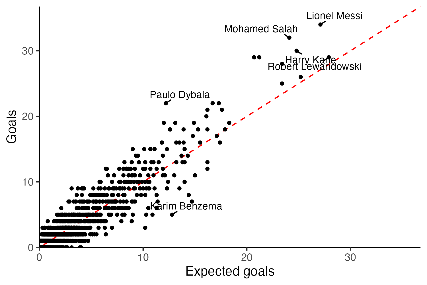
Is it possible to predict which players will consistently overperform or underperform their xG? Of course, xG themselves are designed such that on average, all players will concentrate around the global mean of zero. Consider the aforementioned 2017-2018 season’s distribution of xG over or underperformance, which is described by the following histogram. Most players cluster around the mean of around zero. The scatterplot presents the same concept, with xG on the x-axis and goals on the y-axis. Paulo Dybala overperformed his xG by around 10, while Karim Benzema underperformed by 7.8.
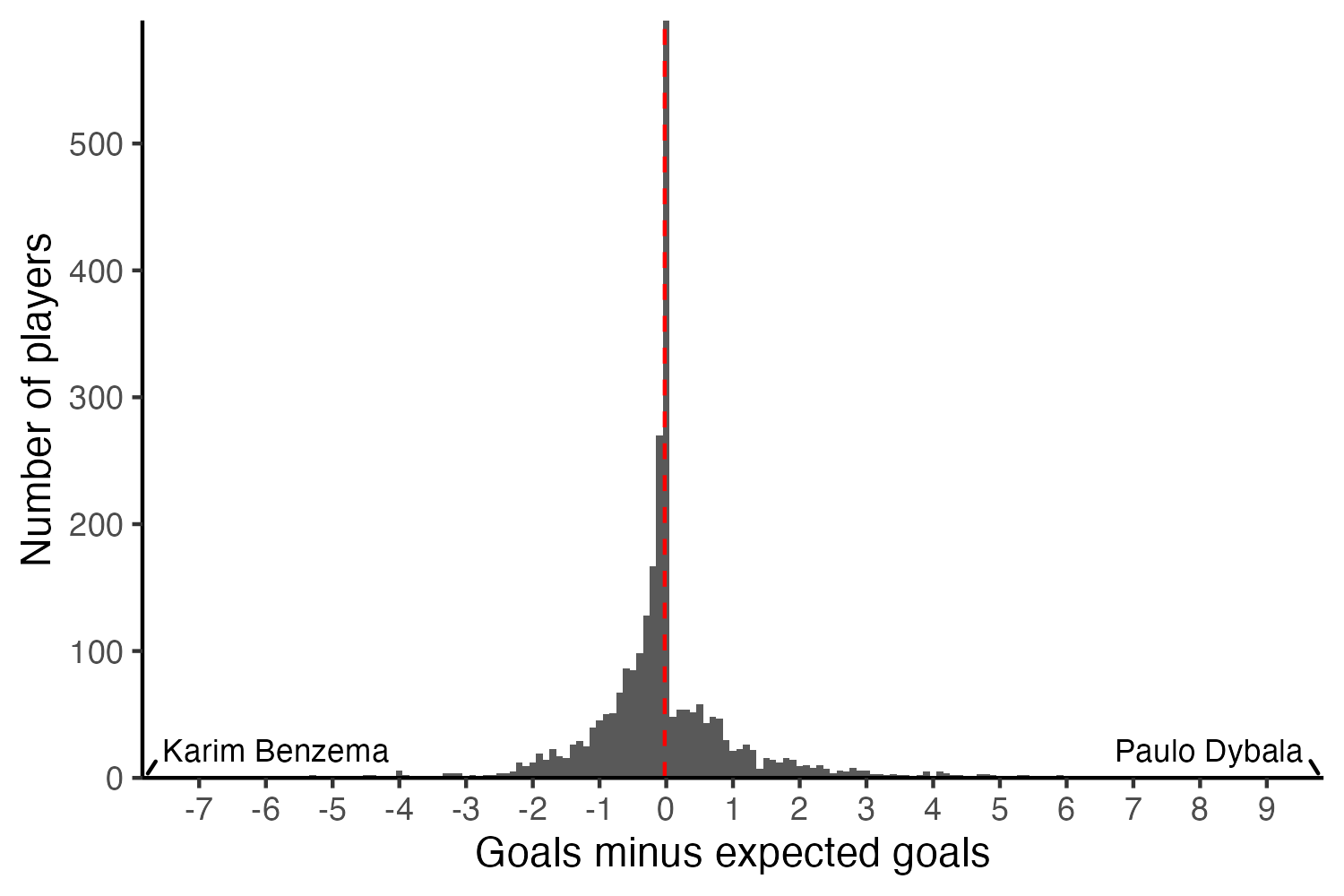
Immediately here, you might see the pitfalls of using xG over or underperformance to characterize a finisher, as is the conventional wisdom, and as friend of the blog Bob Hayes highlights here. The other side of the “well, pretend that you don’t know Messi and just saw his underlying numbers from the 2017-2018 season and didn’t buy him because you expect him to regress down to the mean” is… “pretend you don’t know Benzema and just saw his underlying numbers from the 2017-2018 season and sold him because you didn’t expect him to regress up toward the mean.” Despite my personal allegiances, Benzema is a great finisher and indeed just a few years later went on a historically high xG overperformance in his famous bandaged Champions League run—note the FBref data I’m using are for the top 5 European league competitions only.
A first-level issue here is that Benzema is generating a lot xG (and goals, of course) which is valuable in and of itself barring a theoretically extreme underperformance. One could imagine filtering by a certain number of minutes and calculating some normalized measure of xG over or underperformance that’s normalized by number of minutes played, but let’s set that aside for now because the goal is to fix ideas stylistically here.
The point that I want to make is that while we know that, by construction, the mean of this xG overperformance histogram will be zero. However, less is known about the variance. Is it possible to use information about the variance to gain insights around finishing ability? At the very least, can we learn more about the variance parameters of the xG distribution at a player level? Can we characterize the variance of the distribution at a global level? Do these parameters vary over time?
Let’s decompose a player $i$’s goals scored as a function of their xG generated, some latent “finishing ability”, $\theta_i$, of player $i$ and some noise, $\sigma_i$, that varies across players, modified by a global noise parameter $\eta$.
\[Goals_i = xG_i + \theta_i + \epsilon_i, \quad \epsilon_i \sim \mathcal{N}(0, \sigma_i^2 + \eta^2)\]As the number of observations increases, the relative weight of the player variance parameter should decrease. Intuitively the $\sigma$ represents the idea in words that “we’ve seen enough of Messi” to know that he’s likely to continuously overperform his xG.
There’s an underlying stationarity assumption here that posits that these parameters are time invariant, we could impose some structure by only attempting to estimate this within a single season, though one could consider more fine-grained windows of analysis. However, getting a sense of whether the global variance changes dramatically season-by-season provides suggestive evidence for the plausibility of the stationarity assumption.
Fitting a mutlilevel model in Stan to the data will allow us to estimate individual player level parameters but also global variance parameters, which can give us a sense of how unusual it is, for example, Messi to have overperformed his xG in the 2017-2018 season by about 7, relative to the overall distribution of xG over and underperformance by all other players in Europe’s top five leagues. More importantly, we can also get a sense of whether or not these parameters are predictive of future goal scoring or xG over/underperformance.
data {
  int<lower=0> N;            // number of observations
  int<lower=0> J;            // number of players
  array[N] int player_id_mapped;  // player index
  array[N] int season_id;    // season index
  vector[N] goals;           // goals scored
  vector[N] xG;              // expected goals
}

parameters {
  real mu_theta;             // global mean
  real<lower=0> eta; // global standard deviation
  vector[J] theta_i;           // player-specific finishing ability
  vector<lower=0>[J] sigma_i;  // player-specific noise term
}

model {
  for (j in 1:J) {
    theta[j] ~ normal(mu_theta, sigma_i[j]);
  }

  for (n in 1:N) {
    goals[n] ~ normal(theta[player_id_mapped[n]], eta);
  }
}
So what does our model tell us? Tune in next time I update this post!
-
Let’s set aside potential alternative paths, such as looking at expected goals on target or other advanced stats. I may have another post with some ideas on this based on thinking in terms of counterfactuals sometime soon. ↩